Running and fitting models on naturalistic corpora

Most of XSLmodels is built around controlled cross-situational learning experiments: a handful of words and objects, a designed training order, and a vector of human accuracies to fit with sum-of-squared-error. This vignette is about the other kind of input – naturalistic corpora of caregiver speech paired with the objects present in the scene. There is no human referent-selection data to fit; instead we ask how well a model’s learned word–object matrix recovers a gold-standard lexicon.

Two such corpora ship with the package, imported from the wurwur package:

rollins_corpus$data
#> xslData object with label "Rollins" and condition "CHILDES naturalistic corpus (Frank, Goodman & Tenenbaum, 2009)"
#>   training trials: 619
#>       test trials: 0
#>             words: 416
#>           objects: 22
#>        accuracies: 0
fm_corpus$data
#> xslData object with label "FM" and condition "Frank, Tenenbaum & Fernald naturalistic corpus"
#>   training trials: 4763
#>       test trials: 0
#>             words: 1122
#>           objects: 30
#>        accuracies: 0

rollins_corpus – 619 mother-to-infant utterances from the Rollins corpus in CHILDES; the corpus the intentional Bayesian model of Frank, Goodman & Tenenbaum (2009) was originally fit to.
fm_corpus – the larger Frank, Tenenbaum & Fernald corpus: 4763 utterances, and (unlike Rollins) the speaker’s referential intention is hand-coded for each utterance.

Each is a list, not a bare xslData:

names(rollins_corpus)
#> [1] "data"      "gold"      "reference"
names(fm_corpus)
#> [1] "data"          "intents"       "gold"          "gold_variants"
#> [5] "reference"

$data is the training xslData; $gold is the reference lexicon. Note that words and objects here are the actual strings, not integer ids:

rollins_corpus$data$train$words[[1]]
#> [1] "ahhah" "look"  "we"    "can"   "read"  "books" "david"
rollins_corpus$data$train$objects[[1]]
#> [1] "book"   "bird"   "rattle" "face"
str(rollins_corpus$gold)
#> List of 2
#>  $ words  : chr [1:34] "baby" "bear" "bigbird" "bigbirds" ...
#>  $ objects: chr [1:34] "baby" "bear" "bird" "bird" ...

Running a model

xsl_run() works exactly as it does for experimental conditions – it returns a fitted object whose matrix is the learned word (rows) by object (columns) association matrix.

res <- suppressWarnings(xsl_run(baseline(), rollins_corpus$data))
m <- res$fits[[1]]$matrix
dim(m)
#> [1] 416  22

# co-occurrence counts for one word (this corpus is a picture-book session,
# so the objects are animals and toys -- "moocow", "piggie", etc.)
sort(m["moocow", ], decreasing = TRUE)[1:4]
#>    cow    pig rattle   book 
#>      8      3      3      1

Two things to know:

Ignore res$sse and res$fits[[1]]$perf. Those compare against data$accuracy, which is empty for a corpus. xsl_run() still computes them (falling back to get_perf()), which is where the "longer object length is not a multiple of shorter" warning above comes from – the matrix is not square. It is harmless here; we score against the gold lexicon instead.
The batch model fgt2009() (below) does joint inference over the whole corpus and has no learning trajectory, so control$reps does nothing for it.

Scoring against the gold lexicon

The evaluation helpers take a gold_lexicon = list(words, objects). Because a model’s matrix is real-valued, the score depends on a threshold for counting an edge as “learned”. [get_fscore()] scores one threshold:

get_fscore(m / rowSums(m), threshold = 0.1, gold_lexicon = rollins_corpus$gold)
#> # A tibble: 1 × 5
#>   threshold precision recall fscore specificity
#>       <dbl>     <dbl>  <dbl>  <dbl>       <dbl>
#> 1       0.1     0.143  0.912  0.247       0.977

[get_roc()] sweeps thresholds (row-normalizing the matrix first), and [get_roc_max()] returns the best F-score over that sweep – the standard single-number summary:

roc <- get_roc(m, gold_lexicon = rollins_corpus$gold)
head(roc, 3)
#> # A tibble: 3 × 5
#>   threshold precision recall fscore specificity
#>       <dbl>     <dbl>  <dbl>  <dbl>       <dbl>
#> 1      0       0.0294      1 0.0571       0    
#> 2      0.01    0.116       1 0.207        0.966
#> 3      0.02    0.118       1 0.212        0.967

get_roc_max(m, gold_lexicon = rollins_corpus$gold)
#> [1] 0.3768116
plot_roc(m, gold_lexicon = rollins_corpus$gold)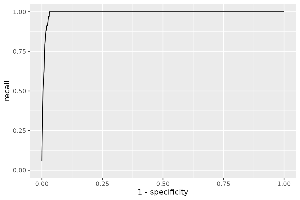

Comparing a few associative models on Rollins:

assoc_models <- list(
  baseline        = baseline(),
  decay           = decay(C = 0.99),
  rescorla_wagner = rescorla_wagner(C = 1, alpha = 0.1, beta = 0.1, lambda = 1),
  fazly           = fazly(lambda = 1e-5, beta = 8500)
)

sapply(assoc_models, function(mod) {
  mm <- suppressWarnings(xsl_run(mod, rollins_corpus$data)$fits[[1]]$matrix)
  round(get_roc_max(mm, gold_lexicon = rollins_corpus$gold), 3)
})
#>        baseline           decay rescorla_wagner           fazly 
#>           0.377           0.343           0.378           0.450

The intentional Bayesian model

fgt2009() is the model built for exactly this problem: it does joint posterior inference over a word–object lexicon for the whole corpus at once, marginalizing the speaker’s referential intention on each utterance. It is a batch MCMC model, so a single run takes seconds to a minute or two on these corpora (much slower than the associative tallies) and xslFit$matrix holds posterior edge marginals P(word names object | corpus).

The gamma parameter matters here. gamma is the probability a word is used referentially. In a controlled experiment every word is a label, so the default is gamma = 1. Naturalistic speech is full of non-referential words (“the”, “look”, “you”, “see”), so a corpus wants the published gamma = 0.1, kappa = 0.05 – otherwise the model is forced to explain every function word as naming something and learns almost nothing.

res <- xsl_run(
  fgt2009(alpha = 3, gamma = 0.1, kappa = 0.05),
  rollins_corpus$data
)
m_fgt <- res$fits[[1]]$matrix

# the learned lexicon: edges with posterior probability > 0.5
edges <- which(m_fgt > 0.5, arr.ind = TRUE)
data.frame(word   = rownames(m_fgt)[edges[, 1]],
           object = colnames(m_fgt)[edges[, 2]],
           prob   = round(m_fgt[edges], 2))
#>       word object prob
#> 1     bear   bear 1.00     # correct
#> 2   bottle   bear 1.00     # "baby bottle" co-occurs with the bear
#> 3  bigbird   bird 1.00     # correct
#> 4     book   book 1.00     # correct
#> 5   moocow    cow 1.00     # correct
#> 6      hat    hat 1.00     # correct
#> 7     oink    pig 1.00     # correct
#> ...                        # 28 edges total

get_roc_max(m_fgt, gold_lexicon = rollins_corpus$gold)
#> [1] 0.454   # MCMC: expect a little run-to-run variation

“Fitting”: sweeping the lexicon-size prior

fgt2009()’s alpha penalizes lexicon size (P(L) proportional to exp(-alpha * |L|)) and has to scale with corpus size: too small gives a diffuse over-large lexicon, too large an empty one. The F-vs-alpha curve is single-peaked, so the right way to “fit” the model to a corpus is a coarse sweep – which is what [fgt2009_sweep_alpha()] does. Pass gold and it reports the best-threshold F-score at each alpha:

sweep <- fgt2009_sweep_alpha(
  rollins_corpus$data,
  alphas = c(2, 4, 6, 9, 14),
  gold   = rollins_corpus$gold,
  gamma = 0.1, kappa = 0.05,
  n_warmup = 50, n_samples = 120      # a lighter sampler for the sweep
)
sweep

The curve rises to a shallow peak around alpha = 2–4 and then falls off as the prior forces the lexicon empty. Take the alpha near the peak; that is the value to report, and the one to use for trial-by-trial predictions ([predict_referent()]) or further analysis. On this small corpus fgt2009 is in the same range as the better associative models (fazly above); its advantage is largest on data with more varied, informative co-occurrence.

The FM corpus and its coded intentions

fm_corpus is used the same way, but it is bigger and comes with extra structure. fm_corpus$intents[[t]] is the object(s) the speaker actually referred to on utterance t – empty for the roughly half of utterances that are non-referential:

fm_corpus$data$train$words[[1]]
#> [1] "and"   "whats" "that"  "is"    "this"  "a"     "puppy" "dog"
fm_corpus$intents[[1]]
#> [1] "dog"

mean(lengths(fm_corpus$intents) == 0)   # fraction non-referential
#> [1] 0.5007348

It also ships three gold lexicons – a hand-curated one plus two auto-derived from the coded intentions at different co-occurrence thresholds:

lengths(lapply(list(curated    = fm_corpus$gold,
                    strict     = fm_corpus$gold_variants$strict,
                    permissive = fm_corpus$gold_variants$permissive),
               `[[`, "words"))
#>    curated     strict permissive 
#>         41         39        116

m_fm <- suppressWarnings(xsl_run(baseline(), fm_corpus$data)$fits[[1]]$matrix)

sapply(list(curated    = fm_corpus$gold,
            strict     = fm_corpus$gold_variants$strict,
            permissive = fm_corpus$gold_variants$permissive),
       function(g) round(get_roc_max(m_fm, gold_lexicon = g), 3))
#> Warning in max(fscores[!is.na(fscores)]): no non-missing arguments to max;
#> returning -Inf
#>    curated     strict permissive 
#>      0.268      0.191       -Inf

The permissive lexicon is larger and easier to hit some of, so absolute F-scores are not comparable across the three – pick one and use it consistently when comparing models.

A quick model comparison

tests/bakeoff_comparison/corpus_gold_comparison.R runs every model once on each corpus and scores the learned matrix against the corpus gold lexicon. It is deliberately not a fitted bake-off: the associative and sampling models use xsl_model_registry()’s starting parameters (calibrated defaults, not re-fit here), and fgt2009() uses gamma = 0.1, kappa = 0.05 with alpha from the two-point heuristic round(7 * sqrt(n / 600)).

Best-threshold F of the learned lexicon vs. the gold lexicon.
model	Rollins	FM
bayesian_decay	0.449	0.450
fazly	0.450	0.407
fgt2009_rsa	0.395	0.421
fgt2009	0.385	0.421
uncfam_sampling	0.394	0.360
multi_sampling	0.394	0.352
uncfam	0.377	0.360
uncfam_gamma	0.377	0.360
uncfam_elimination	0.377	0.360
uncfam_attention	0.377	0.351
propose_but_verify	0.409	0.318
softmax_rl	0.376	0.336
pursuit	0.400	0.307
guess_and_test	0.396	0.304
baseline	0.377	0.268
minerva2	0.359	0.267
rescorla_wagner	0.312	0.290
decay	0.320	0.272
kalman_filter	0.303	0.211
uncfam_predictive	0.235	0.185
todam	0.174	0.048
tilles	0.080	0.048

rem() is left out: at roughly 11 minutes per simulation on FM, averaging the 50 simulations used for the other stochastic models isn’t practical.

Reading the table:

bayesian_decay and fazly come out on top (F around 0.45 on both corpora), with fgt2009 close behind.
fgt2009 trades recall for precision. On FM its precision is ~0.71 against ~0.15–0.34 for the others: the geometric size prior makes it commit to a small, mostly-correct lexicon rather than a large noisy one. Whether that is the right tradeoff depends on what you want the lexicon for.
The RSA layer makes no difference on FM (fgt2009 == fgt2009_rsa): at alpha = 20 the learned lexicon is sparse enough that no word names two co-present objects, so the pragmatic speaker reduces to the literal one.
The middle of the pack is a tight cluster around F = 0.35–0.40: the uncfam variants, the two sampling versions (which are meant to approximate uncfam()), and the hypothesis-testing models (propose_but_verify, pursuit, guess_and_test), which do relatively better on Rollins than on FM.
Every model now runs on both corpora, but several needed fixes to get there. The sampling/RL models were built for controlled experiments of a few dozen trials; running them on 4763 naturalistic utterances exposed a memory blow-up (xslControl()’s keep_traj = FALSE default), an error on the many non-referential utterances with no objects present, and latent bugs: softmax_rl() and guess_and_test() compared a sampled guess to object positions vs labels; guess_and_test() mishandled a word repeated within one utterance; tilles() coerced its labels with as.integer() and returned an unnamed matrix; and propose_but_verify() and pursuit() drew hypotheses from the wrong set on utterances with a single object present (common in both corpora).
tilles and todam still learn diffuse lexicons at their default parameters: their best threshold is 0, i.e. no threshold separates correct pairings from the rest. For tilles, fitting its parameters lifts F to ~0.40–0.43 (below), so read the low default score as “this parameterisation doesn’t transfer”, not “the model is broken”.

Fitting to a corpus

tests/bakeoff_comparison/corpus_gold_fits.R goes a step further: for each model it runs a (parallel) DEoptim search over the model’s parameters, maximizing the same best-threshold F against the gold lexicon (these corpora have no accuracy vector, so xsl_fit()’s SSE objective does not apply). fgt2009() is fit by an alpha sweep instead. uncfam_sampling(), multi_sampling(), pursuit(), and the episodic-memory models are left at defaults – averaging many simulations per DEoptim evaluation over 4763 utterances is impractical.

Best-threshold F: registry default vs. fit to the corpus.
model	Rollins_default	Rollins_fitted	FM_default	FM_fitted
bayesian_decay	0.449	0.465	0.450	0.560
fgt2009	NA	0.452	NA	0.529
fgt2009_rsa	NA	0.447	NA	0.515
softmax_rl	0.360	0.447	0.299	0.429
fazly	0.450	0.463	0.407	0.412
uncfam_gamma	0.377	0.450	0.360	0.425
uncfam_attention	0.377	0.420	0.351	0.417
tilles	0.080	0.427	0.048	0.400
uncfam	0.377	0.420	0.360	0.388
guess_and_test	0.372	0.440	0.292	0.368
uncfam_elimination	0.377	0.404	0.360	0.400
propose_but_verify	0.400	0.438	0.325	0.360
rescorla_wagner	0.312	0.389	0.290	0.343
decay	0.320	0.382	0.272	0.288
kalman_filter	0.303	0.382	0.211	0.275
uncfam_predictive	0.235	0.333	0.185	0.233

Fitting lifts every model, and by a lot for the ones whose registry defaults were tuned on controlled experiments: tilles (+0.35 on both corpora), softmax_rl (+0.09 / +0.13), uncfam_predictive (+0.10 / +0.05).
bayesian_decay fit to FM reaches F = 0.56 – clearly the strongest result – with fgt2009 next at 0.53. fazly barely moves (its defaults were already near-optimal for these corpora).
uncfam_gamma() is the best uncfam variant once fit (0.45 / 0.43, vs 0.42 / 0.39 for uncfam()), with a fitted familiarity exponent of 1.56 on Rollins and 0.77 on FM – so neither corpus is consistent with familiarity entering linearly, but they disagree on the direction. uncfam_elimination() gains less (0.40 / 0.40).
fgt2009_rsa fit (best of an alpha sweep) lands just below fgt2009 (0.45 / 0.52 vs 0.45 / 0.53) – the pragmatic layer neither helps nor hurts once alpha is chosen, because the fitted lexicon is still too sparse for a word to name two co-present objects.
The fitted parameters are in corpus_gold_fits.rds. kalman_filter’s sigma2_obs lands high (1511 / 1923, against an upper bound of 2000), but that is a plateau, not an estimate: the three Kalman parameters share a scale redundancy and the F landscape is flat in sigma2_obs above a few hundred. Read its fitted sigma2_obs as “large”.

References

Frank, M. C., Goodman, N. D., & Tenenbaum, J. B. (2009). Using speakers’ referential intentions to model early cross-situational word learning. Psychological Science, 20(5), 578–585.

Frank, M. C., Tenenbaum, J. B., & Fernald, A. (2013). Social and discourse contributions to the determination of reference in cross-situational word learning. Language Learning and Development, 9(1), 1–24.

George Kachergis

2026-10-16